Model-Preserving Adaptive Rounding with YAQA

We’re excited to announce YAQA (Yet Another Quantization Algorithm), a new weight-only LLM post-training quantization method that quantizes models to directly preserve the original model’s outputs. YAQA is quantizer-agnostic, meaning that it can be used with both hardware-accelerated datatypes and special memory-bound quantizers like QTIP. Across a wide range of models and quantizers, YAQA consistently reduces the KL divergence to the original model by >30% over existing rounding algorithms, resulting in state of the art performance on downstream tasks.

Post-Training Quantization

The main goal of post-training quantization is to produce a smaller model whose outputs are as close as possible to the original model’s. Formally, given some high-precision model parameters $\theta^*$ and a set of representable low-precision points $C$, we want to minimize the distance between the original model outputs $M(\theta^*, X)$ and quantized model $M(\theta, X)$ over some inputs $X$ sampled from an input distribution $\mathcal{D}$ and model architecture $M$:

$$\hat \theta \gets \text{argmin}_{\theta \in C} \mathbb{E}_{X \sim \mathcal{D}} D_{\text{KL}}(M(\theta^*, X) \| M(\theta, X))$$

Unfortunately, exactly solving $\hat \theta$ is intractable. Most existing quantization algorithms such as LDLQ, GPTQ, and AWQ instead try to solve a proxy layerwise minimization problem by independently minimizing the immediate activation error for each linear layer in $M$. For a linear layer $y=xW^T$, this can be written as 

$$\text{argmin}_{W \in C} \mathbb{E}_{x\in\mathbb{R}^n \sim \mathcal{D}}\|x(W^* - W)^T\|_F^2 = \text{argmin}_{W \in C} \mathbb{E}_{x \sim \mathcal{D}} \ \text{tr}((W^* - W)x^Tx(W^* - W)^T).$$

Although this objective works well in practice, it does not consider the effect of quantization on layers after $W$ and vice versa. As such, minimizing it does not necessarily reduce the KL to the original model. 

A Better Proxy Error

Instead of minimizing the immediate layerwise activation error, YAQA directly minimizes the KL by using a near-optimal Kronecker-factored approximation of each linear layer’s Hessian with respect to the KL. If this seems complicated, don’t worry, it’s not nearly as bad as it sounds. Consider the second order expansion of the KL minimization problem for a linear layer $W \in \mathbb{R}^{m \times n}$:

$$\text{argmin}_{W \in C} \mathbb{E}_{X \sim \mathcal{D}} D_{\text{KL}}(M(\Theta^*, W^*, X) \| M(\Theta^*, W, X)) \approx \frac{1}{2} (W - W^*)^T (\nabla_{W^*}^2 L) (W - W^*)$$

Here, $L$ is the KL divergence to the original model, so we can ignore first order terms since $\nabla_{W^*} L = 0$ (the KL of a distribution to itself is 0). This leaves $H = \nabla_{W^*}^2 L$, or the full Hessian of the linear layer. $H \in \mathbb{R}^{mn \times mn}$ has $O(10^{12})$ elements, which makes it too large to manifest. However, due to some nice properties of the KL divergence, we can tractably compute Hessian-vector products with $H$, which lets us find low-rank approximations of $H$ that we can subsequently use for quantization.

YAQA makes use of two well known facts from linear algebra to quantize with $H$. First, the Hessian of the $KL$ is the Fisher Information Matrix (FIM). The FIM is given by $\mathbb{E}[\text{vec}(\nabla_{W^*} \ell) \text{vec}(\nabla_{W^*} \ell)^T]$, where $\nabla_{W^*} \ell$ can be obtained by backpropping through a specially constructed loss. The important thing here is that individual samples of the FIM’s expectation can be computed with the cost of a single backprop, which means we can tractably compute Hessian-vector products with the FIM. Second, we utilize the fact that the Kronecker product of two matrices $A \otimes B$ is equivalent to a reshaped rank-1 product. This means that we can find the optimal Kronecker-factored approximation of $H \approx H_O \otimes H_I$ by finding the optimal rank-1 approximation of $H$, which can be done with power iteration and the aforementioned Hessian-vector products.

Finding $H_O$ and $H_I$

We wish to find $H_O$ and $H_I$ such that $H \approx H_O \otimes H_I$. Since $H_O \otimes H_I$ is a reshaped rank-1 matrix, we can find the optimal $H_O, H_I$ that minimizes 

$$\|H - H_O \otimes H_I\|_F^2$$ 

with power iteration. Power iteration computes the following updates

$$H_O \gets \frac{HH_I}{\|H_I\|_F^2} \hspace{2cm} H_I \gets \frac{H^T H_O}{\|H_O\|_F^2}$$

Where $H$ is reshaped from $(mn, mn) \to (m^2, n^2)$. The convergence rate of power iteration is a function of the spectral gap of $H$, which is empirically high for LLMs.

In YAQA, we present two different Hessian sketches for $H_O$ and $H_I$. Our first sketch (sketch A in the paper) uses a biased, low variance estimate of $H$ for power iteration. Our second sketch (B in the paper), which we describe below, uses an unbiased but higher variance estimate of $H$ for power iteration. B generally produces better models since it is unbiased, at the cost of being more expensive than A. 

Recall from before that $H$ is given by the Fisher Information Matrix

$$H = \mathbb{E}[\text{vec}(\nabla_{W^*} \ell) \text{vec}(\nabla_{W^*} \ell)^T],$$

where $\ell$ is a specially constructed loss (see paper for details) and the expectation is taken over independent samples. Since we are operating in LLM-land, tokens within a sequence are not independent due to attention. This means that we must calculate the expectation over entire sequences instead of tokens, which reduces the achievable sample size for a fixed compute budget. While this isn’t catastrophic, it does limit us to either running fewer rounds of power iteration with more samples or using fewer samples and doing more power iteration – using many samples and doing multiple rounds of power iteration would simply be too expensive.

In sketch B, we directly compute the result of $H_O$ and $H_I$ after one round of power iteration with $H$ in a single pass over a dataset by using an identity initialization. In some sense, this gives us a near-optimal compute-quality tradeoff for calculating $H_O$ and $H_I$ since we can power iterate on both while only making one pass over the devset. In contrast, updating $H_O$ first and then updating $H_I$ would require two passes over the devset, making Hessian sketching twice as expensive. 

Sketch B initializes $H_O$ and $H_I$ to the identity matrix $I$. If we expand out the power iteration equation with the definition of the FIM, we get

$$H_I \gets \frac{\mathbb{E}_{s \sim D}\left[(\nabla_{W^*}\ell)^T H_O (\nabla_{W^*}\ell)\right]}{\|H_O\|_F^2} \hspace{0.25in} H_O \gets \frac{\mathbb{E}_{s \sim D}\left[(\nabla_{W^*}\ell) H_I (\nabla_{W^*}\ell)^T\right]}{\|H_I\|_F^2}$$

which gives $H_I = \mathbb{E}_{s \sim D}\left[(\nabla_{W^*}\ell)^T (\nabla_{W^*}\ell)\right] / m$ and $H_O = \mathbb{E}_{s \sim D}\left[(\nabla_{W^*}\ell)(\nabla_{W^*}\ell)^T\right] / n$ after one round of power iteration with an identity initialization. Since the only thing required to compute $H_O$ and $H_I$ is $\nabla_{W^*} \ell$, we can compute $H_O$ and $H_I$ with a modified backward pass, which composes with distributed training frameworks like FSDP to scale to hundred-billion parameter models.

Quantizing with $H_O$ and $H_I$

Now that we have $H_O$ and $H_I$, we want to quantize models with them. In YAQA, we propose a new adaptive rounding algorithm that uses linear feedback from $H_O$ and $H_I$ to quantize linear layers with theoretical guarantees. YAQA’s rounding algorithm is in some sense a natural extension of QuIP’s LDLQ rounding algorithm, where we have feedback along the output dimension in addition to the input dimension in LDLQ. In fact, we show that LDLQ is actually a special case of YAQA’s rounding algorithm that is theoretically worse than YAQA.

Consider the family of adaptive rounding algorithms that performs the update

$$W_{i, j} = \mathcal{Q}\left({W^*}_{i, j} + a_{i}^T({W^*}_{:i, :j} - W_{:i, :j}) b_{j} + a_{i}^T({W^*}_{:i, j} - W_{:i, j}) + ({W^*}_{i, :j}-W_{i, :j})b_{j}\right)$$

where $a_i$ is the $i$-th column of a strictly upper triangular $m \times m$ matrix $L_O$, $b_j$ is the $j$-th column of a strictly upper triangular $n \times n$ matrix $L_I$, and $\mathcal{Q}$ is a quantizer that performs nearest or stochastic rounding. Ignoring the cursed indexing, what this essentially does is quantize an entry in $W^*$ based on the entry itself and the error from quantizing entries below or to the right of it. In the example below of a 4x5 weight matrix, the blue entry (1, 2) is rounded with feedback from all the red entries ($i \ge 1$ or $j \ge 2$).

The final result of performing these updates is a $W$ that satisfies 

$$W = \mathcal{Q}\left({W^*} + L_O^T\Delta WL_I + L_O^T\Delta W + \Delta W L_I\right),$$

which lets us reason about how to choose $L_I$ and $L_O$. In general, if we choose $L_I$ and $L_O$ to be the triangular part of the LDL decomposition of $H_I$ ($H_I = L_ID_IL_I^T$ for unit lower triangular $L_I$ and diagonal $D_I$) and $H_O$, then we can bound the error of this rounding procedure by something $O(tr(D_I)tr(D_O))$. 

So far, we haven’t actually said anything about how useful this bound is. As far as we care, $H_O$ and $H_I$ could be any positive definite matrices. However, with some math, we can show that 

$$\Delta W H \Delta W^T \le \|H\|\left(\|\Delta W\|_F^2 \sqrt{2-2c} + \frac{tr(D_O)tr(D_I)}{\|H_I\|\|H_O\|} \sigma^2 \right)$$ 

where $c$ is the cosine similarity between $H$ (the actual Hessian with respect to the KL, which is too expensive to manifest) and $H_O \otimes H_I$. This means that closer $H_O \otimes H_I$ is to $H$ directionally, the better our rounding algorithm will minimize the second order expansion of the end to end KL, which is what we care about. Thankfully, power iteration also maximizes the cosine similarity, so our $H_O$ and $H_I$ should have pretty high cosine similarity.

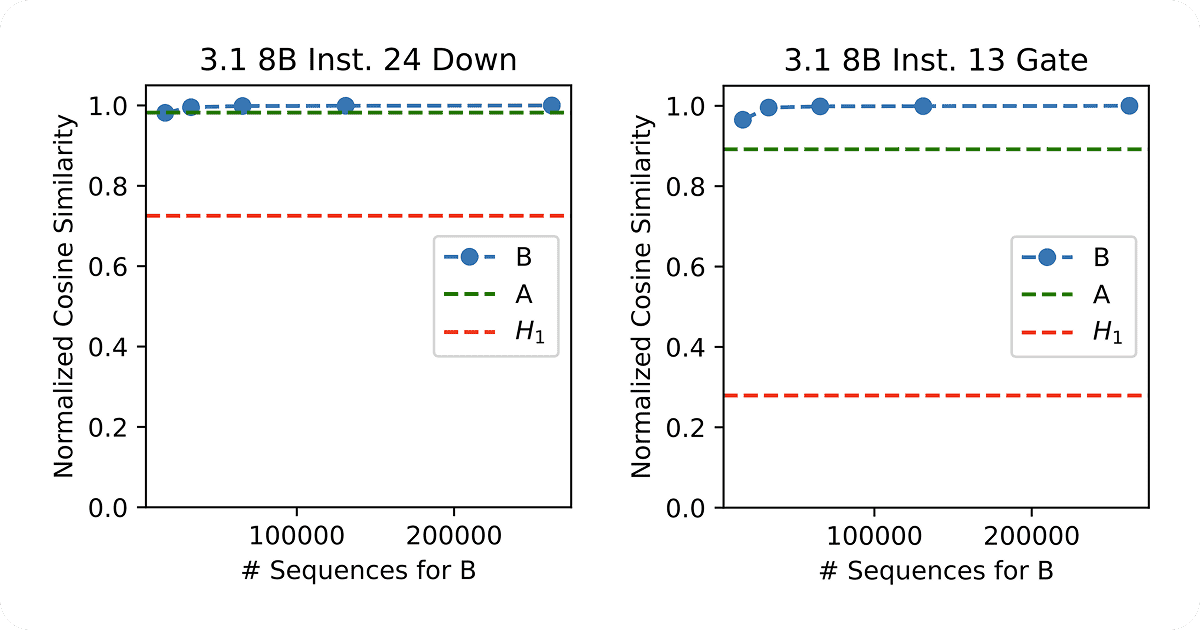
Indeed, we can verify this by computing the relative cosine similarity (ignoring the $\|H\|$ term since that is fixed and also intractable to compute exactly) between various $H_O, H_I$ and $H$. We can also check how much better YAQA is than LDLQ from QuIP, which minimizes the layerwise problem $\text{argmin}_{W \in C} \mathbb{E}[\|x(W^* - W)^T\|_F^2]$. As it turns out, LDLQ, which is equivalent to GPTQ, is simply YAQA with $H_I \gets \mathbb{E}[x^Tx]$ and $H_O \gets I$. In the two plots below, both sketches B (from above) and A (in the paper) have much higher cosine similarity than LDLQ’s Hessian estimate ($H_1$), so adaptive rounding with YAQA should better minimize the end to end KL divergence.

Experiments

We empirically verified YAQA’s performance by quantizing Llama and Gemma models with various quantizers. Across most models, we saw that YAQA reduced the KL divergence to the original model by a factor of ⅓, which translated to state of the art downstream performance. Since YAQA works with any quantizer, these results are applicable to both compute and memory-bound inference scenarios. 

The table below shows the effect of YAQA with the QTIP quantizer, incoherence processing, and no finetuning. At all bitrates and model sizes, both YAQA A and B significantly reduce the KL divergence to the original model.

The table below shows the same setup but this time with recovery finetuning. Since existing methods don’t directly minimize the KL, they usually employ some sort of finetuning during and after quantization to better minimize the KL. Finetuning still works with YAQA, but has less of an effect since YAQA directly minimizes the KL. Regardless, YAQA still maintains a considerable gap over LDLQ and achieves state of the art downstream results.

Finally, we compared YAQA against quantization aware training (QAT) methods that use expensive training recipes to simulate the effect of quantization during training. Like YAQA, QAT methods generally try to directly minimize the KL to the original model. Although QAT recipes are usually not open source, Google has thankfully released an official QAT version of Gemma 3 12B Instruct, which should be representative of what a top industry lab can achieve with QAT. Our experiments show two interesting results. First, the QAT model somehow outperforms the original model on downstream tasks. Second, even without finetuning, both YAQA models achieve a lower KL than the QAT model and are closer on downstream tasks (but worse than the original as expected). All this suggests that the QAT process is actually producing a considerably different model, whereas YAQA is preserving the original model.

Using YAQA

Peeling a yaca is hard. However, we’ve made it easier by open sourcing our code, precomputed Hessians, and some prequantized models. Alternatively, you should probably just use Together AI’s high-performance APIs, which are fast, cheap, and easy to use.